
This article is kindly donated by Mike Tilby and first appeared in the SMEE Journal issue October 2018.
An electronically controlled Mono-tube boiler - Part 1
This project started several years ago, long before I joined the Society of Model & Experimental Engineers (SMEE). It was triggered by information gathered from a search on the Internet for guidance on how to automatically control the water level in a model boiler. That search took me to a description of a model that was to completely change the course of my model engineering activities. The model in question was described in a long series of messages under the heading ‘Flash Steam Plant Control’ on the very good model boating forum Model Boat Mayhem (MBM). The topic had been started by someone calling himself Flashtwo and it described a flash steam boiler that was completely controlled by electronic circuits based around the devices called microcontrollers. The steam plant described by Flashtwo on the MBM forum was eventually installed in a radio controlled model boat called Vital Byte which was later described in two articles in Engineering in Miniature under FlashTwo’s real name of Ian Gerrard. (Ref. 1).
Looking back, I wish the excellent series of SMEE articles Electronics for Model Engineers by Gareth Hughes (Ref. 2) had been available to me when I started out on this project since, when I first read the messages by Flashtwo, I had never even heard of microcontrollers. I now realise I had been surrounded by them for many years since, for the last few decades they have been key components of many domestic and work-place appliances and every modern car probably contains a few dozen of them.
However, this project seems to have a different slant to other projects that I have seen mentioned in The SMEE Journal or on the Digital Group web-pages. Electronics-related projects seem to have mostly concerned building or enhancing workshop tooling, and the only exception I have seen in recent years was a robot by Mike Kapp and Alan Wragg (Ref. 3). However, being located 300 miles north of the Society’s head quarters, I have probably missed things. In this project, as in the above-mentioned robot, electronics has been integrated into an actual model.
In the concluding part of his Electronics for Model Engineers series Gareth Hughes wrote “I hope you have been able to see the power and usefulness that even a basic knowledge of electronics can give to the model engineer.” (Ref 4). The present series of three articles is submitted in the hope that it serves to illustrate and reinforce that message and it certainly does not pretend to show particularly good ways to achieve the goals of the project. So if they trigger suggestions for how things could be done better then that will be most useful.
Mono-Tube (AKA Flash steam) boilers
In case some readers are not familiar with mono tube (or flash steam) boilers, I should just explain that the term refers to boilers that are basically the equivalent of what is commonly called a combi-boiler in a domestic heating system, or what used to be known as an Ascot instant water heater. A mono tube boiler has no steam or water reservoir but consists of a long length of tube coiled into one of a number of possible compact shapes. Water is pumped into one end of the tube while flame(s) from one or more burners are directed through the coils and eventually turns the contained water into steam. Unfortunately, the term 'Flash Steam' is applied to many mono-tube boilers which are not operated on the ‘flash’ principle. In the latter, the tubes are heated empty to some given high temperature and then water is pumped in which flashes instantly into steam. Pretty well all the boiler designs in “Experimental Flash Steam” by Benson & Rayman (Ref 5) are actually mono-tubes rather than flash designs.
These days, stainless steel tubing is most commonly used but in my case it is 16 ft of 1/4 in. o.d. copper tube that I bought from Bonds O’ Euston Road, about 50 years ago. I have fond memories of that old shop with its many small wooden drawers against the back wall and its dark wood counters above glass display cases full of enticing models and tools. Back then I coiled the tube into its present shape but never completed a boiler because life’s worldly pressures took over. But the embryo boiler persisted through several different lofts, as well as in my ageing grey matter. Eventually it came in very handy for this project which uses electronic components that would have seemed like science fiction when the tube was initially purchased. (See Fig 1 - the boiler with the top of the casing removed.)

Examples of mono-tube boilers
When a mono-tube boiler is running stably, water is pumped into one end of the tube at the same rate as the steam is delivered from the other end. In the past such boilers featured prominently in round-the-pole steam hydroplane racing. That particular racing fraternity tended to use the term ‘Flash Steam’ rather than ‘mono-tube’ which is probably the origin of the current misconception. Back-issues of Model Engineer describe numerous record-breaking hydroplanes where boiler pressures of a few thousand psi could be produced. Our local authority has banned this activity on its ponds on grounds of safety. However, the safety concerns relate to the high speeds attained by the boats (over 120 mph) and not the high boiler pressures. In fact model-sized mono-tube boilers have not been subject to any safety regulations or inspections since they are not classified as pressure vessels. They pose no significant explosion risk because the volume of steam and super-heated water contained in them is so small. However, superheated steam is particularly hazardous and these days model engineering societies may require certain basic safety features1.
Actually a large proportion of our electricity supply relies on what are essentially large sophisticated mono-tube boilers since all modern power stations that burn fossil or bio-fuels use boilers constructed out of relatively small diameter steel tube, although these are generally called ‘once-through boilers’.
Combining electronics with traditional model engineering can be very enjoyable and, of course, this is simply making hobby engineering more akin to the contemporary real world - where electronic and mechanical engineering are closely integrated in so many everyday objects - from cookers to cars.
Microcontrollers
Back in the 1970s I used to enjoy writing programs for analysis of laboratory data using what was then probably the best small computer – a BBC Master with a Torch second processor. At that time I felt I knew roughly what was going on in the computer and it was easy to connect it to pieces of equipment. But, as computers evolved and PCs with Windows operating systems took over, everything became so complex that now I no longer really know what goes on inside the box. That background is perhaps why, once I learnt a little about them, microcontrollers quickly appealed to me since each one is basically a mini-computer that is specifically designed to interact with the outside world. In fact, in many ways, a single microcontroller can be more powerful than a BBC computer and can easily be fully understood since there is no complex operating system to get in the way. This also means they rarely freeze-up and so they can be left operating indefinitely - unlike some PC applications. On top of all this, they only cost a couple of quid each! Use of microcontrollers by hobbyists took off with the arrival of versions based on so-called flash memory which means they can be easily and repeatedly re-programmed. Before that, people had to be very certain of their programming skills before burning a new program into them irreversibly.
The microcontrollers used by many hobbyists are made by the electronics company Microchip. Like several other manufacturers, Microchip makes very many ranges of these devices, and each range contains huge numbers of different versions. Microchip’s microcontrollers were originally called Peripheral Interface Controllers, now universally abbreviated to PIC. The latest microcontrollers are becoming ever more sophisticated but the PICs that I have used are relatively simple ones and are classed as ‘mid-range’ devices. In general, microcontrollers certainly look rather unimpressive (Fig. 4) but nevertheless each one can be programmed to perform a huge range of functions. The fact that the basic data sheet for the simple type that I use runs to 400 pages is an indication that they are capable of a wide range of activities.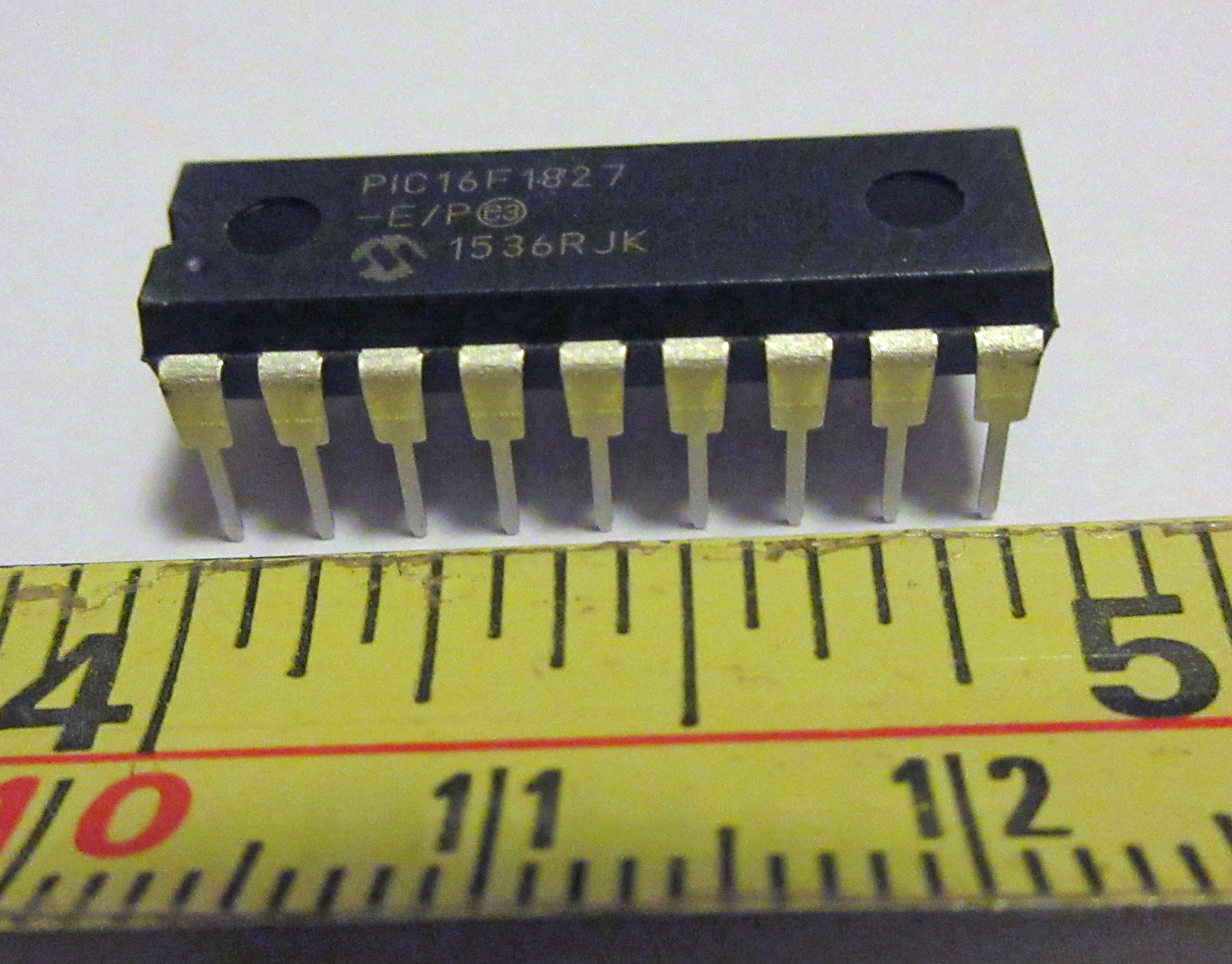
In case anyone is interested, the type of microcontroller used in this control system is PIC16F1827. Programs were worked out initially as flow diagrams in PowerPoint and then written in assembly language using the free PC software from Microchip called MPLAB IDE. Next, the PICs were programmed using a Pickit 3 programmer and finally the inevitable bugs were investigated and fixed, initially with circuits built on a bread-board.
Boiler control systems
My steam plant was inspired by Ian's system but all mechanical parts, electronic circuit boards and microcontroller programs have been designed completely independently. Both systems carry out the same overall control whereby a boiler feed pump is driven by a DC motor and this is controlled electronically to run at the desired speed. Temperature of steam leaving the boiler is measured by a thermocouple and compared to the temperature that one wishes to achieve. Ian’s system uses a gas burner and a control valve is adjusted using a commercial servo. A PIC controls this servo so as to attain the desired target steam temperature.
Ian's system is more sophisticated in several ways. Also, it works well and is installed in the fine and completely finished model launch. In contrast, my system is really just a test bed to see what I could achieve and it is the result of a very steep learning experience. It is too bulky to be used in a model boat and is certainly not a nicely finished model that would inspire admiration of workmanship etc. Nevertheless these articles focus on my own efforts in the hope that they might trigger ideas for other projects and suggestions for improvements.
Microcontrollers that use a bus
In Ian’s design, all key control processes are performed by one central PIC whereas my system evolved in a different direction since several key functions are performed by separate PICs. Ian called my system a ‘distributed control system’ which seems good to me because that label sounds quite impressive.
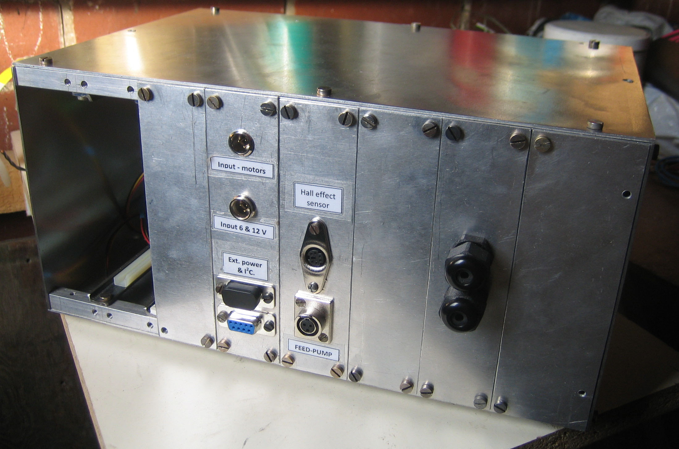
Each of the five PICs in my system is on its own circuit board. One of these PICs, called the Master, is in overall charge of the others which are called Slaves. The Master and two of the slave PICs are housed in the main electronics box (Fig. 5). 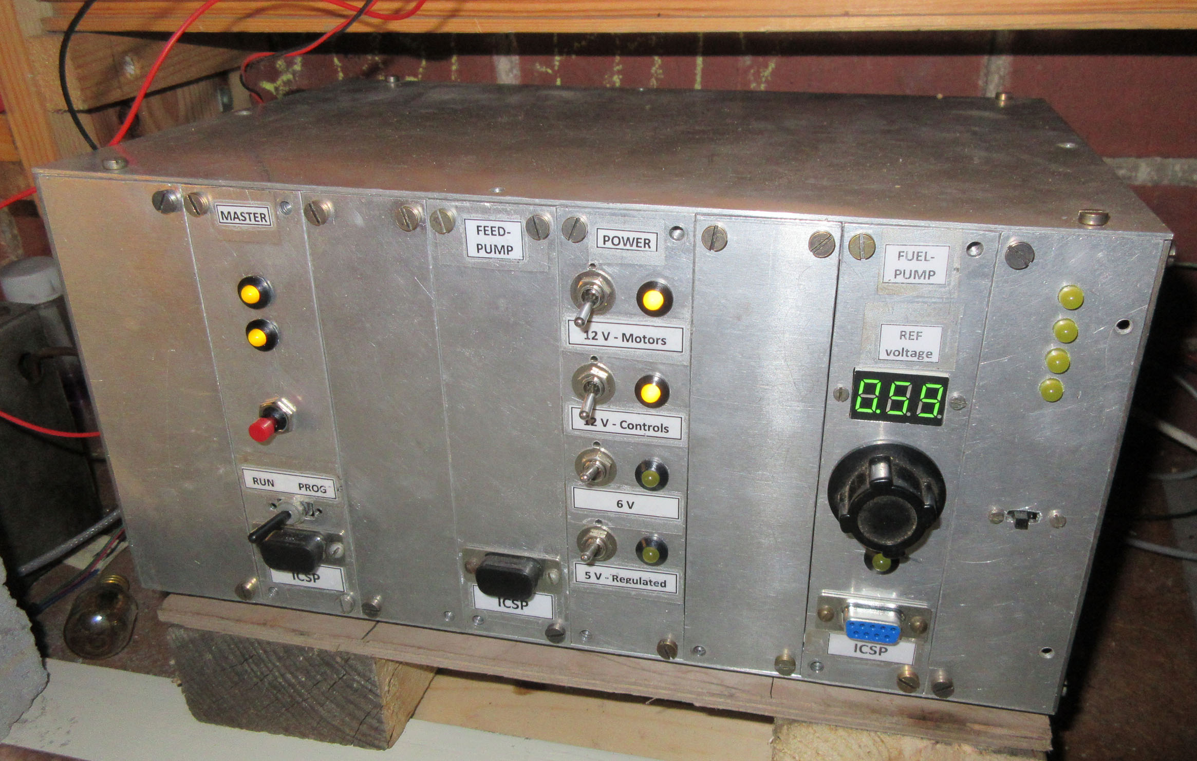 This also contains additional circuit boards for controlling power to the pump motors.
  The other two slave PICs are housed in a small semi-portable box which has a four line liquid crystal display (LCD) for showing various values and control options. That box also has a number of buttons and switches for input of commands and settings. (Fig. 6).
The master PIC is connected to all the slaves by two wires called a bus. In this case it is called an I2C bus because the signals sent along it conform to a scheme of this name that is an industry standard originally developed by the Philips company back in the 1980s. 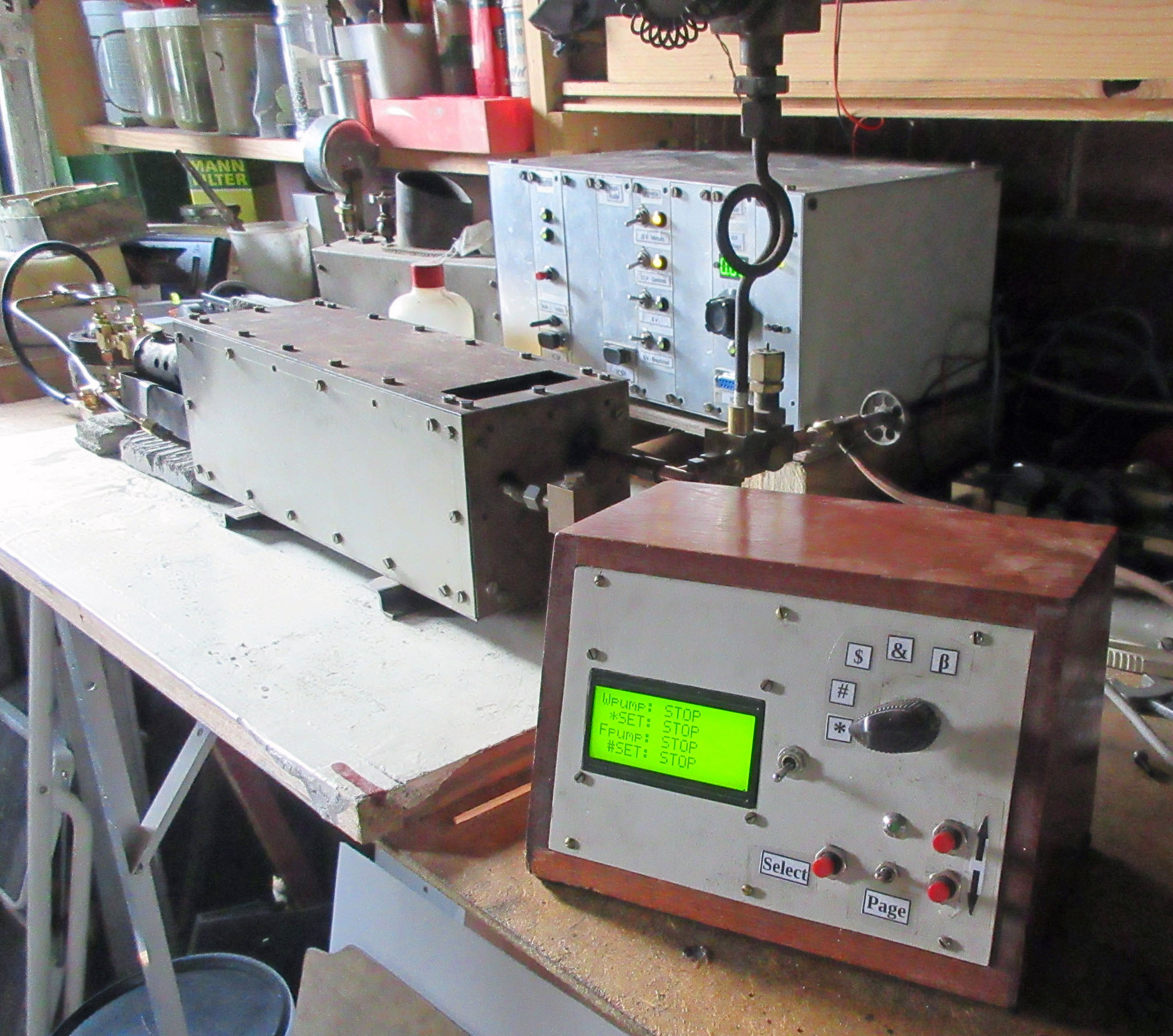 In the basic type of I2C bus, one master microcontroller can individually talk to up to 127 different slaves. Each message transmitted from the master starts with a number which identifies the slave that is being addressed. The master can then send a stream of data to that slave over the bus and can also receive data sent back from the slave. Many types of device other than PICs can be connected to an I2C bus. In this boiler control system the only additional device is a so called real time clock (RTC). As presently configured, the master PIC simply instructs the RTC to provide, over a separate connection, a timing pulse every second. However, it could also read out real time and date information if that were ever required. Another useful addition to the bus could be a memory device.
I use one of these in a different project where it is used to record and read back quite large amounts of data to extend the limited data memory that is built into the PIC itself. The I2C bus was developed to allow communication between devices located fairly close to each other, but I find that it works well via a lead several feet long connecting the main box to the small display box.
Control system
The overall system is summarized in Fig. 7 which makes it look more complicated than it really is.  Basically an electric feed pump delivers water to the boiler at the speed sent from the master PIC to the feed-pump control PIC. The temperature of steam coming from the boiler is measured every few seconds and if it is too low or too high then the Master PIC automatically sends an instruction to the fuel pump PIC telling it to increase or decrease the fuel-pump speed. All current settings are stored in the PIC flash data memories and can be adjusted by pressing appropriate switches connected to the input PIC. Values such as the target and actual pump speeds and steam temperature can be shown on the LCD display. The next article will describe the feed-pump and how its speed is measured and controlled.
References
- Ian Gerrard, 2012. Monotube boiler control system parts 1 and 2. Engineering in Miniature, Feb p 262 – 265 & 269; March p 328 – 330.
- Gareth Hughes (2015) Electronics for Model Engineers Part 1 The Journal, vol 23 (5) Oct: 32 – 35.
- Mike Kapp and Alan Wragg (2006) A robot made for BBC competition - photo in Work on the Table, The Journal, vol. 14 (6) Nov 10 - 11.
- Gareth Hughes (2017) Electronics for Model Engineers Part 8 The Journal, vol 25 (5) Oct: 31 – 35.
- Benson J.H & Rayman A.A (1973) Experimental Flash Steam, Model and Allied Publications Ltd, Hemel Hempstead.
Footnote 1: The SBA requires any boat attending an SBA Event that uses a mono-tube boiler to have an SBA approved certification as well as the normal SBA PL insurance.
 An electronically controlled mono-tube boiler - part 2
In Part 1 the journey into the world of electronically enhanced model engineering was outlined and the nature of the boiler and its control was introduced. After installing the old copper coil in a proper housing, the next task was to design and make the ancillaries; a feed pump and the electronic circuitry to control it.
Feed pump
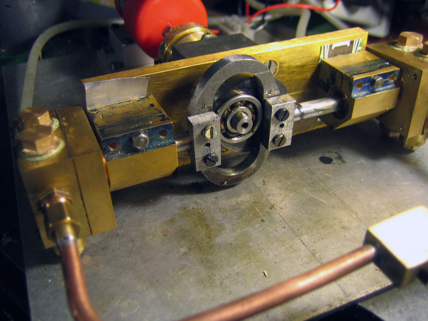
Excessive pulsation in the pumping rate could affect boiler performance so the pump is of the Scotch yoke type with two barrels such that water is delivered as the ram moves in each direction (Fig. 1).
The pump is driven by a 12V DC motor and its speed is measured with a Hall effect sensor which detects the passing of a small magnet that rotates on the pump shaft (Fig. 2).
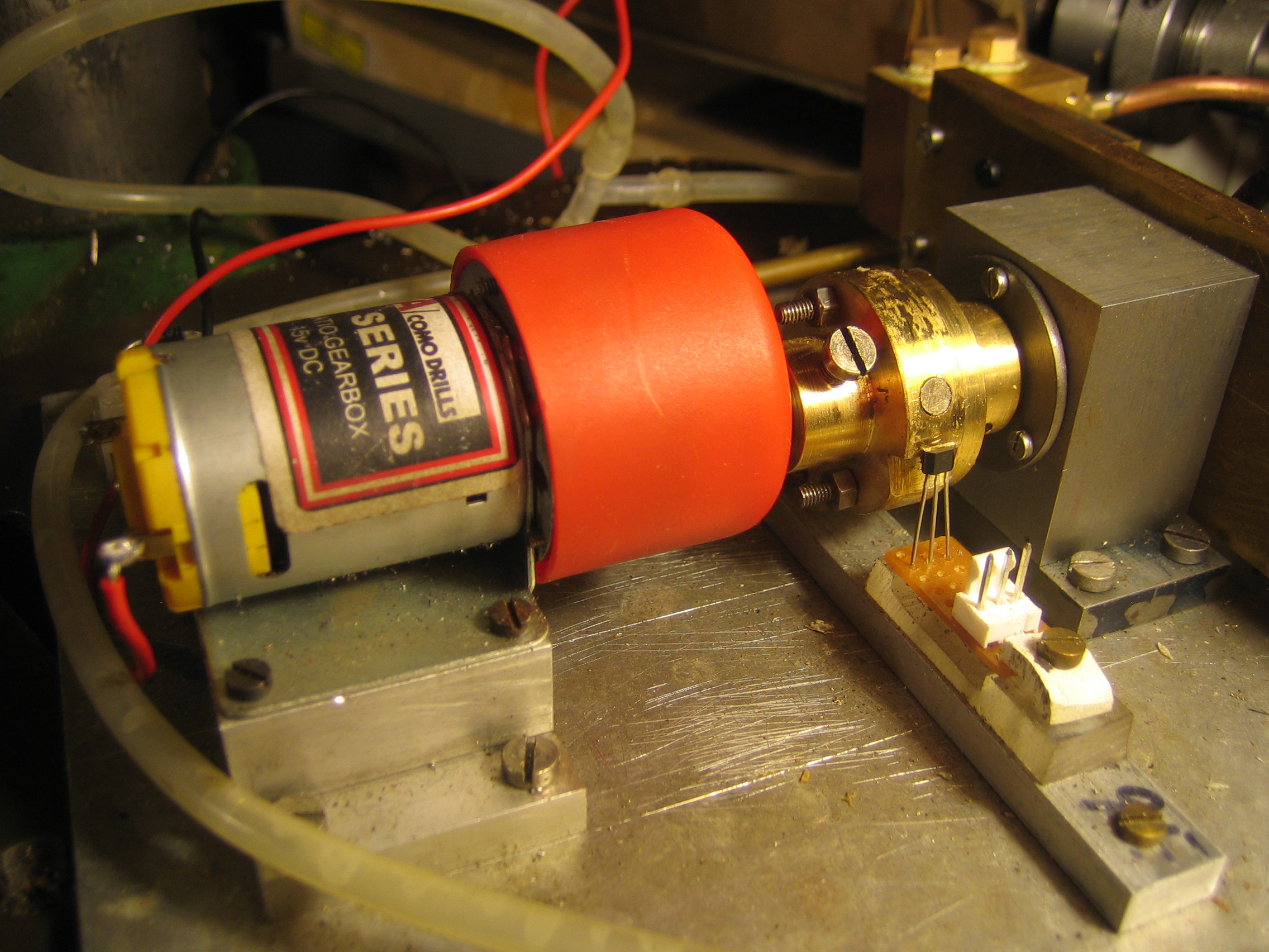
Every time the pump shaft rotates this sensor sends a signal to the slave PIC that is dedicated to controlling the pump. This PIC measures the time elapsing between each signal and calculates the rpm. The resulting value is sent to the master-PIC. If appropriate, the master-PIC then relays the rpm value to the display PIC, as shown in Fig. 3.

Data input/output
The need to display the pump speed brings us to the liquid crystal display (LCD). The information shown on the LCD is determined by a dedicated slave PIC which receives information from the master-PIC. It is necessary to be able to show more information than can simply be fitted onto the 4-line LCD so the information displayed at any one time can be changed between a number of different pages, each of which suits a different purpose. The page shown in Fig. 3 is for manual control of the feed-pump while other pages are for control of the fuel pump, setting up the temperature control parameters, etc. The information repeatedly sent to the display-PIC by the master-PIC includes a page number and a series of values. From the page number the display-PIC works out the appropriate text characters to send to the LCD device.
The numeric values sent by the master PIC to the display PIC must be appropriate for the particular page. These values are sent in the standard form that makes sense to electronic devices, i.e. in 8- or 16-bit binary code. Binary coded values are easily sent down the wire by rapidly switching the voltage between +5V (binary 1) and 0V (binary 0). These 8- or 16- bit values have to be translated by the display-PIC into signals suitable for sending to the LCD device. This entails firstly converting a binary code into a code that indicates the correct sequence of decimal digits that can be easily read by us humans. The result of this conversion is a value called binary coded decimal. The display-PIC programme then uses these values to instruct the LCD device which characters it must display. Also the display-PIC has to be programmed to include a decimal point, where necessary, and to work out where to put it. The PIC also has to determine which explanatory text needs to be displayed. Then it must send appropriate signals, in the correct order, to the LCD to make it display all those characters. This is done by setting 12 output pins on the PIC to various combinations of 0 or +5 volts. These pins are connected to 12 input pins of the LCD device.
Closely related to display of data is the need to allow the user to make adjustments to settings such as the pump speed or to change the page being displayed. Such inputs are achieved by use of a number of switches on the small control/display box (Fig. 3). The value chosen for alteration is selected by either the position of the rotary switch or by pressing the ‘Page’ switch. The ‘up/down’ and ‘Select’ buttons are used to increment or to select the chosen value. All these switches are connected to the input-PIC which interprets the meaning of the switches according to the current page being displayed. It then sends the appropriate information back to the master-PIC.
Speed regulation
As described more fully by Gareth Hughes (Refs 1 & 2), the speed of the motor could be controlled by varying the voltage sent to it but this method would be difficult to achieve without wasting energy. Electronic switches are good for switching current full ON or full OFF but any intermediate state results in the control circuit getting hot. Instead, it is very common to control a DC motor by pulse width modulation (PWM). This is a grand sounding title for a simple process of switching the voltage rapidly full ON and full OFF thousands of times a second with control being achieved by changing (i.e. modulating) the width of the ON time compared to the OFF time. The current that flows through the motor does not change as rapidly as does the voltage because of the induction effects of the motor windings. The main result is that the average current varies with the voltage pulse width.
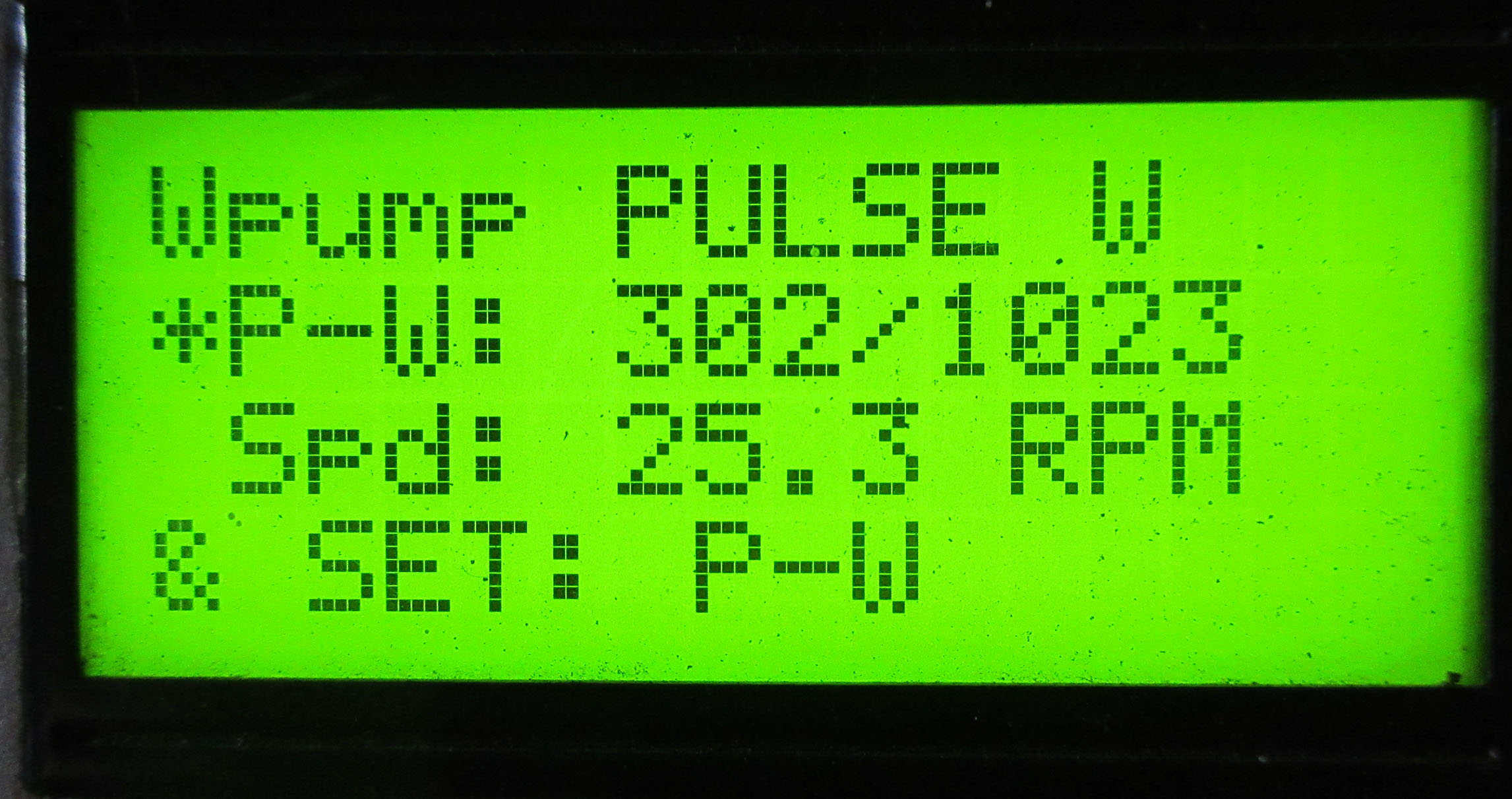
The motor control PIC can easily perform this PWM control function while also measuring and calculating the RPM and communicating with the master PIC. The pump can be controlled in one of a number of modes which is shown in the bottom line of the display (Fig. 4). This can be changed by turning the rotary switch (Fig. 3) to the ‘&’ position, then using the ‘up/down’ buttons and finally pressing the ‘select’ button. One of the pump modes is control by manual adjustment of pulse width. Fig. 4 shows the display for using this mode. If the rotary switch (Fig. 3) is set to ‘*’ then use of the ‘up/down’ buttons directly changes the pulse width that is displayed in the second line (compared to the maximum possible value of 1023). The speed that is calculated from the signals sent from the Hall-effect sensor is displayed in the third line.
In addition to the above functions the feed-pump-PIC has yet another quite complicated task to perform. Instead of manually adjusting pulse width, a desired rpm for the feed pump can be chosen (via the control/display box). This desired rpm is relayed to the master PIC and hence to the motor control PIC which then has to automatically work out how to change the PWM pulse width so as to either speed up or slow down the pump so as to attain the desired speed.
PID feed-back control
In some machines a motor speed can be simply changed by altering the setting of the pulse width to a value that one knows gives the required speed. But with a boiler feed pump the power needed to drive the pump at the desired rpm depends upon the boiler pressure and friction in the pump. Therefore one really needs a feed-back control which adjusts the power to keep the pump turning at the correct speed independently of variation in these factors.
A whole complicated field of study has evolved that deals with control of machines etc. In the simple terms that I can understand there are three basic control strategies in common use. Let us deal with these in relation to the boiler feed-pump. The first, method is known as proportional (P) control whereby the PIC repeatedly calculates by how much the actual speed differs from the target speed. Then it increases or decreases the power supplied to the motor (i.e. it adjusts the PWM setting) by an amount proportional to the size of the error.
Thus, if the pump is far too slow then a big increase in power is made but if it is only slightly too slow then a small increase in power is made. This sounds fine but it does not always work very well in practice since a small error in speed can persist and never get corrected. The second method is called integrative control (I). In this case, the errors for several successive cycles of measurement and analysis are added together. This has the effect that, over time, a small error will give rise to a sufficiently large cumulative control value as to make an impact. The third control method is known as differential (D). In this, the rate at which the pump speed approaches the target speed is calculated. If it is approaching very rapidly then the rate of change is decreased and vice versa. In many situations these three controls are all used together to give an optimum response and this is then referred to as PID control. From his previous experience with control systems Ian Gerrard predicted that the D component would not be needed and his control employs just P and I.
In my system the PIC that controls the feed-pump motor can be instructed to operate in feed-back control mode. In that mode, every time the PIC calculates a new rpm value (i.e. each time it receives a signal from the Hall effect sensor), it performs the PID calculations. It then uses the result to automatically adjust the pulse width so as to either speed up or slow down the pump motor to attain the desired speed. There are sensitivity settings (coefficients) for each of the P, I and D calculations and these can be adjusted via the input/display box (the values Kp, Ki and Kd in Fig. 5). In practice I found that the best results were obtained with the D element turned completely off just as was predicted by Ian.
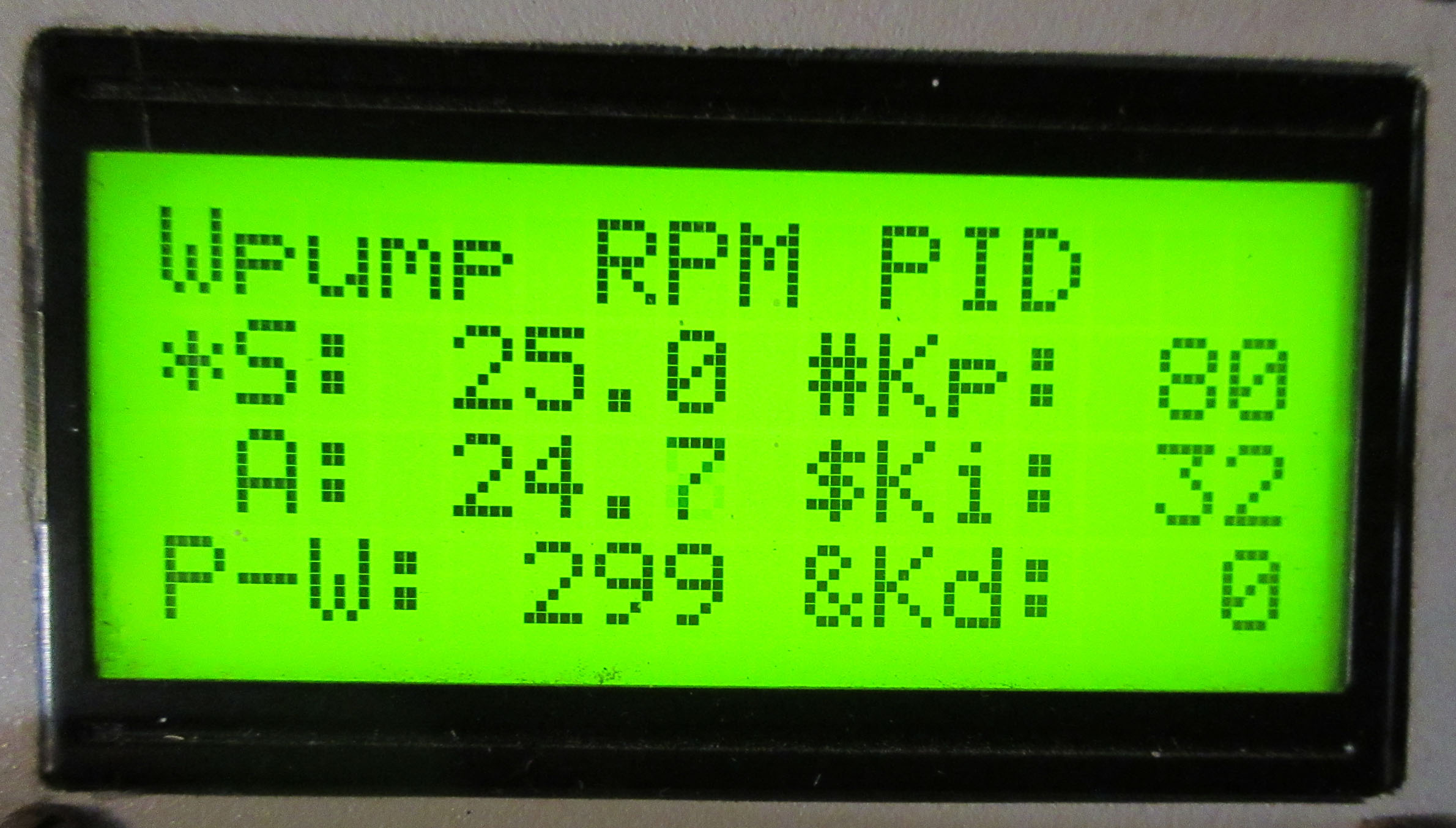
As shown in Fig.5, the pulse width, set speed and actual speed can all be displayed at the same time. It is pleasing to watch the control system perform its adjustments. If, for example, the set speed is increased by a large amount, the pump initially starts to accelerate quite rapidly and often goes slightly too fast. It then starts slowing down more gradually and may under-shoot but by a much smaller amount. This process proceeds until the speed is at the set value and during operation it is generally held to that speed plus or minus 0.1 rpm.
Practicalities of electronics
“A change is as good as a rest” and the tasks of designing and building the pumps, burners and boiler made welcome changes from the challenges of designing and building the circuit boards and writing the PIC codes (and vice versa) I started out using strip-board but eventually bit the bullet and got to grips with making etched boards. Designing the circuits and layout of tracks on the boards was done with the free but comprehensive and well supported programme DesignSpark from RS components. Etching the copper clad boards should have been straightforward, however, the big problem I encountered was how to transfer the printer output of the design onto the copper so as to provide a non-porous etchresist pattern. A huge amount of advice and instruction is available on the internet and much of this describes how to print an image of the tracks with a laser printer and then transfer the toner to the copper-clad board so that the toner forms a barrier to the etching solution.
This all sounded great but I struggled for ages to find a method that worked reliably for me. Several methods that were described as being reliable proved useless in my hands. Eventually I ended up adapting various methods to give a procedure that seems to work reliably, is very cheap and gives solid tracks that are ‘good enough’ for my purposes.
Gas burner
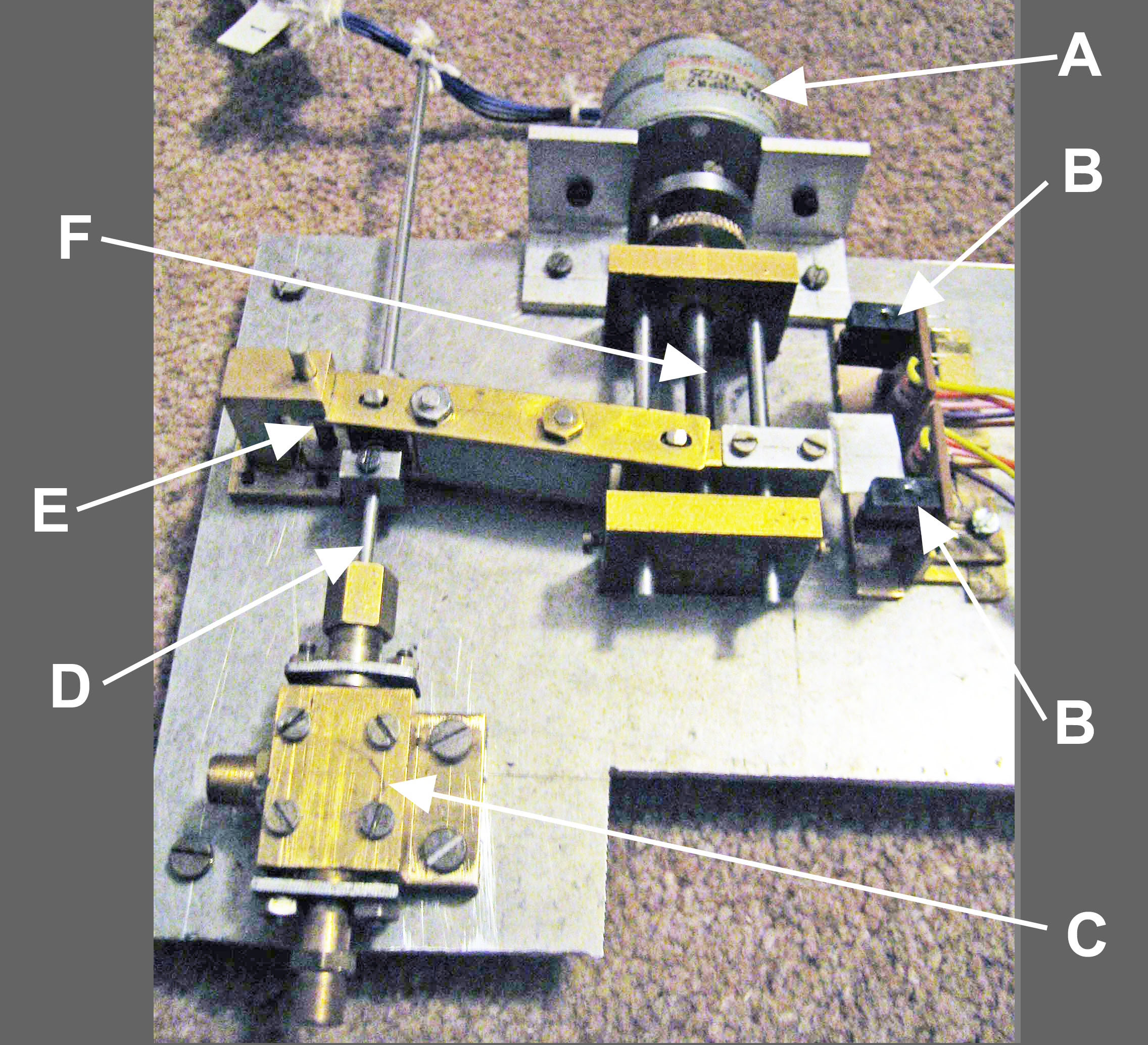
Initially the boiler was fired by bottled gas, however, achieving a design of burner that actually worked was another task which wasted a considerable amount of time. Having achieved a useful burner, attention was then turned to making a needle valve that could be controlled electronically. The opening/closing of the valve is controlled by a stepper motor (Fig. 6). I had collected a few stepper motors from old printers etc over the years and was pleased to at last find a use for one of them. As described more fully by Gareth (Ref. 3) stepper motors do what the name says and rotate in a series of steps, with the direction determined by which of their coils are newly activated compared to the coils that were active in the previous step. Widely used simple stepper motors are of the type known as unipolar. This name signifies that electric current only ever flows in one direction through any of the windings. This type of motor commonly has 4 coils and 5 or 6 leads and they are easy to use with a PIC. Each motor coil is controlled by one of the output pins of the PIC and the minimum that the PIC has to do is turn each of 4 output pins on or off in the correct sequence. Each of these pins controls power supplied to a motor winding via a power transistor – one for each coil. As voltage across a motor coil is switched, high voltages can be generated by induction effects and so these transistors must be protected from damage by suitable diodes. The stepper motor turns a threaded rod thereby moving a nut. Movement of the nut is limited by optical sensors that send a signal to the PIC (Fig. 6). Movement of the valve rod is coupled to the nut by a 4:1 lever, thereby giving a fine adjustment for the gas valve.
The valve worked well and I had fun building and programming all this, but it turned out that gas was a poor choice of fuel because I could not generate a sufficiently powerful flame for the boiler and this problem was exacerbated by the fact that, as gas was used, the temperature and pressure in the small gas container dropped. I have since learnt that this is a common problem and people at my local model boat club have devised effective ways around it. But by the time I learnt about this I had already attempted something different.
An electronically controlled paraffin blowlamp
Compared to gas burners, paraffin blowlamp type vaporising burners are cheaper to run and can more easily provide a really powerful flame. They have been widely used for ‘flash steam’ hydroplanes where paraffin is often forced into the burner by having a pressurised fuel tank, as in a traditional plumber’s blowlamp. However, in the more powerful models the steam engine often drives a fuel pump (i.e. in addition to the boiler feed-pump).
In this arrangement, the faster the engine goes, the faster that water and fuel are pumped to the boiler and burner, respectively. When things are set up correctly, water and fuel outputs keep pace with each other and with engine rpm. These plants usually run flat-out in the hope of breaking speed records and the fuel pumps operate at high rpm. My plan was to drive a fuel pump by an electric motor in the hope of achieving a controllable rate of combustion.
Stepper motor pump drive
A uniform delivery seemed particularly important when trying to maintain a constant flame intensity at low pumping speeds, but even with a two-ram pump the flow rate would still vary throughout each stroke. This is because, at constant rotational speed, the ram speed is maximum in the middle of each stroke and slows down to zero at each end. Concern about this aspect and the risk that the flame could go out triggered the decision to adopt an additional strategy to help maintain constant rates of fuel delivery.
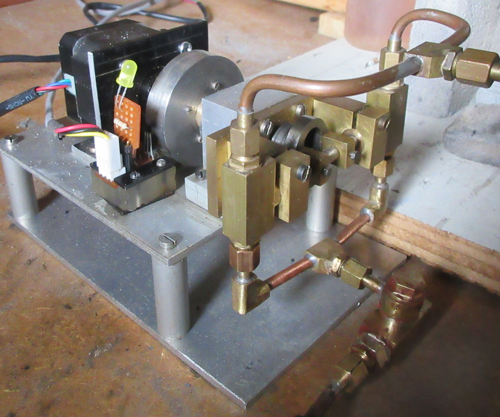
The pump (Fig. 7) was to be driven by a stepper motor - mainly because I like playing with them. Such motors might not be a sensible option for installation in a model boat but this was only intended as an exploratory project. An advantage of using a stepper was the possibility of varying the shaft speed during each rotation. So the control system was designed to make it possible to use a mode of operation where, during each revolution, the pump speed increases from slowest at mid-stroke to fastest at the end of each stroke. By suitably programming the PIC the times between steps can be calculated to give an almost constant ram velocity whilst maintaining the desired average rpm. However, to achieve this, it is necessary to let the PIC know the ram position so it can synchronise the changes in stepping times. That was accomplished using another Hall effect sensor.
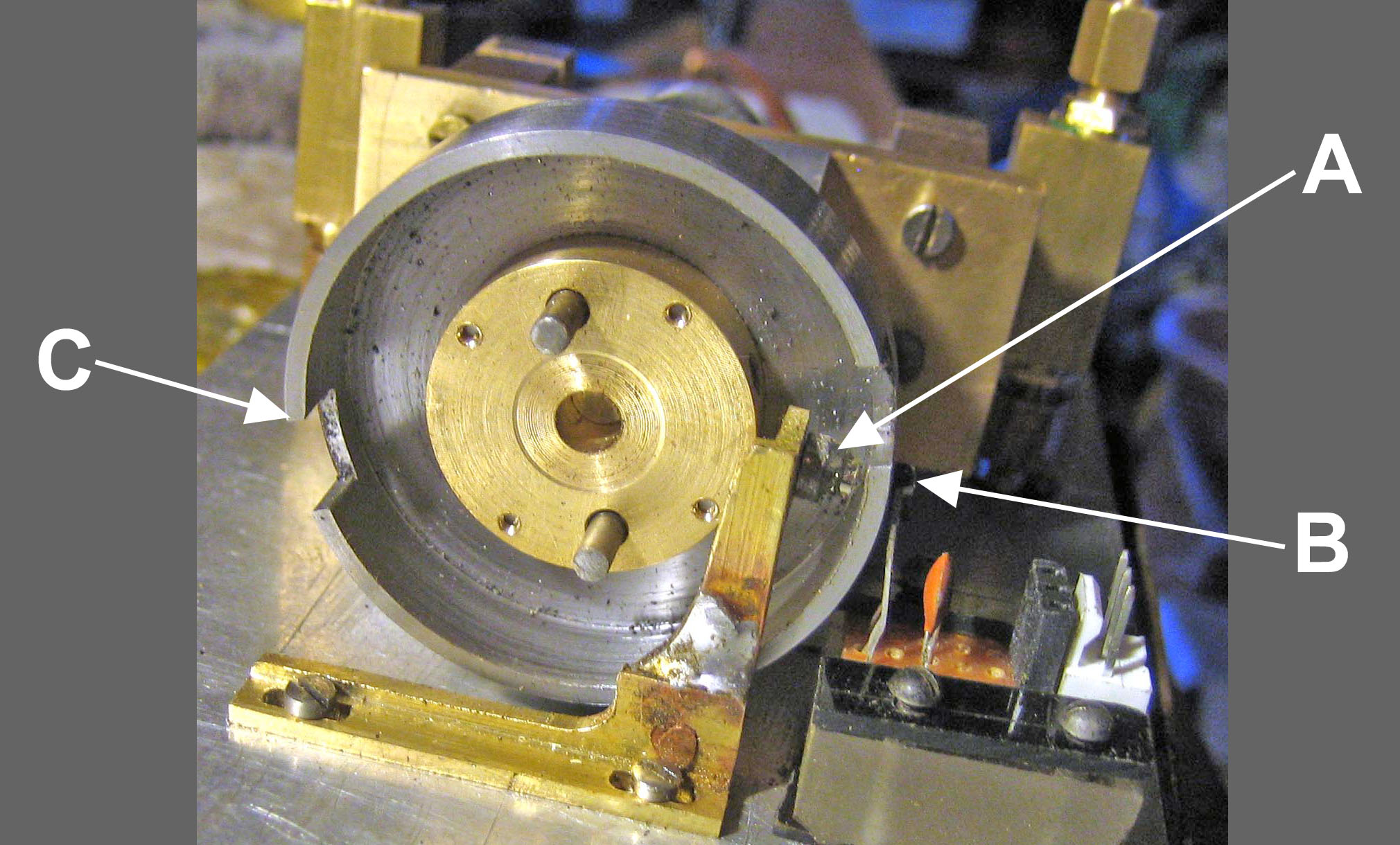
This time the magnet and sensor both remain stationary and a steel ring is placed between them. The ring is fixed to the pump shaft and has two slots cut into it (Fig. 8). As each slot passes between sensor and the magnet the magnetic field detected by the sensor changes and that causes it to send a signal to the PIC. This was just like the operation of the distributor in my old Peugeot car. Initially another unipolar stepper from an old printer was used but this seemed to lack sufficient torque for maximum pumping rates, so it was upgraded.
A better stepper
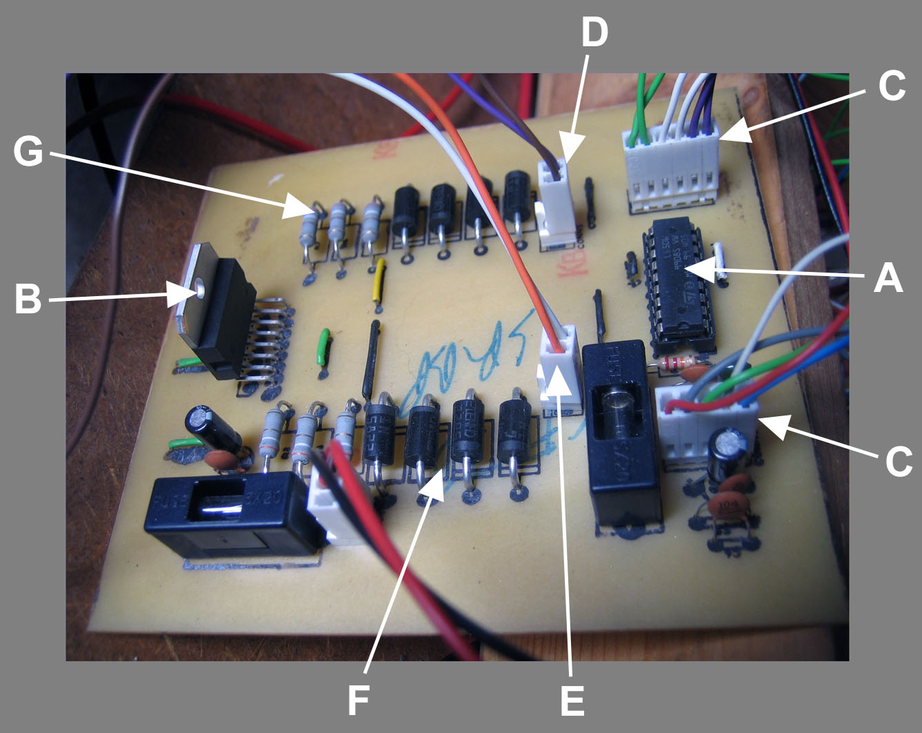
For the greatest range of size, power and quality of motor it seems necessary to use a type of stepper motor known as bipolar. In a bipolar motor, electric current can be made to flow in either direction through each winding. This makes more effective use of the windings but greatly complicates the electronics needed to power the motor since each winding has to be controlled by four transistors arranged in a so-called bridge circuit. Bridge circuits were described by Gareth (Ref. 1) who explained how incorrect switching of the transistors could lead to a dead short circuit between the positive and negative power tracks, which would destroy the components. Therefore my motor was controlled using a specialised stepper motor controller device (L6506, Fig. 9) which controls the switching of the power transistors in a way that makes such errors impossible. This device also measures the current that flows through each motor winding and prevents it from exceeding a maximum level. The reason such current sensing is used will be described in the next and final part of this series.
To be continued.
References
1. Gareth Hughes (2016) Electronics for Model Engineers Part 4 The Journal, vol 24 (3) Jun: 14 – 18.
2. Gareth Hughes (2016) Electronics for Model Engineers Part 6 The Journal, vol 24 (6) Dec: 25 – 29.
3. Gareth Hughes (2017) Electronics for Model Engineers Part 8 The Journal, vol 25 (5) Oct: 31 – 35.
An electronically controlled boiler - part 3
by Mike Tilby
More on a journey into the world of electronically enhanced model engineering.
So far this tale has reached the stage where an electrically pumped paraffin blowlamp was attempted and the initial unipolar stepper motor drive was replaced with a bipolar motor. It was also mentioned that the controller for this motor included a means to monitor the current flowing through each of the two motor windings.
You may wonder why such a refinement is needed since, if the supply voltage were appropriate for the motor, then the current would not increase beyond a safe level. The reason for this refinement stems from the fact that in any electric motor, after the voltage across a coil is turned on, the current does not reach its maximum level instantly. Instead the phenomenon of induction acts to slow down the rate of current increase. In a stepper motor this can lead to the situation where the next step starts before the current in the present step has had a chance to attain its maximum level. This is important because it is the current that determines the strength of the electromagnetic field and so failure to attain maximum current means that the maximum torque exerted by the motor is reduced. If stepping is very slow then this is not a problem since each step lasts long enough for the current to build up to maximum. However, for efficient rapid stepping the way around the problem is generally to supply a voltage much higher than the ‘rated’ voltage of the motor. This causes the current to increase rapidly at the start of each step. However, the voltage must be turned off as soon as the current reaches the desired level otherwise the motor will be damaged.
To measure the current flowing through the motor winding a low value resistor is included in each power circuit. From Ohm’s law (voltage = current x resistance) The voltage drop across this resistor is proportional to the current flowing at any moment. For each of the two motor windings the stepper controller compares this voltage drop to a reference voltage. When the voltage drop across the resistor equals the reference voltage the controller cuts off the supply to that winding. Then, after a very short delay, the voltage is turned on again until the current once again reaches its set limit. This process is repeated many times a second until the next step is activated. In my system the reference voltage is set by a potentiometer and is displayed on a cheap mini digital voltmeter. (The LED display of the voltmeter and the associated potentiometer knob can be seen towards the right-hand end of the electronics box in the upper photo of Fig. 5 in the first article of this series).
The task of making my own stepper control board may not seem the most sensible approach. Recently I have heard that, for a few pounds one can buy ready made stepper control boards that are more sophisticated than my effort (Ref. 1). However, I find it pleasing to make as much as possible from scratch and have learnt much from the experience. The fuel pump PIC receives instructions from the master PIC which tell it the rpm required and whether or not to use the variable step timings (see part 2). The fuel pump PIC then repeatedly works out which windings and current direction should be activated and when to do this. It sends appropriate signals to the L6506 stepper controller and that device then turns on the appropriate power transistors which are contained in a dual MOSFET bridge device (L298, Fig. 9 in part 2).
As explained by Gareth Hughes (Ref. 2), it is possible that a stepper motor can miss steps if resistance to turning is too great. Since the pump has a Hall effect sensor set up to detect rotation (see part 2) it is easy for the PIC to monitor the number of steps between each signal from this sensor and determine if this is more than it should be. An LCD display page can be chosen which shows, for the latest ten half-rotations, which ones, if any, required extra steps.
Burner performance.
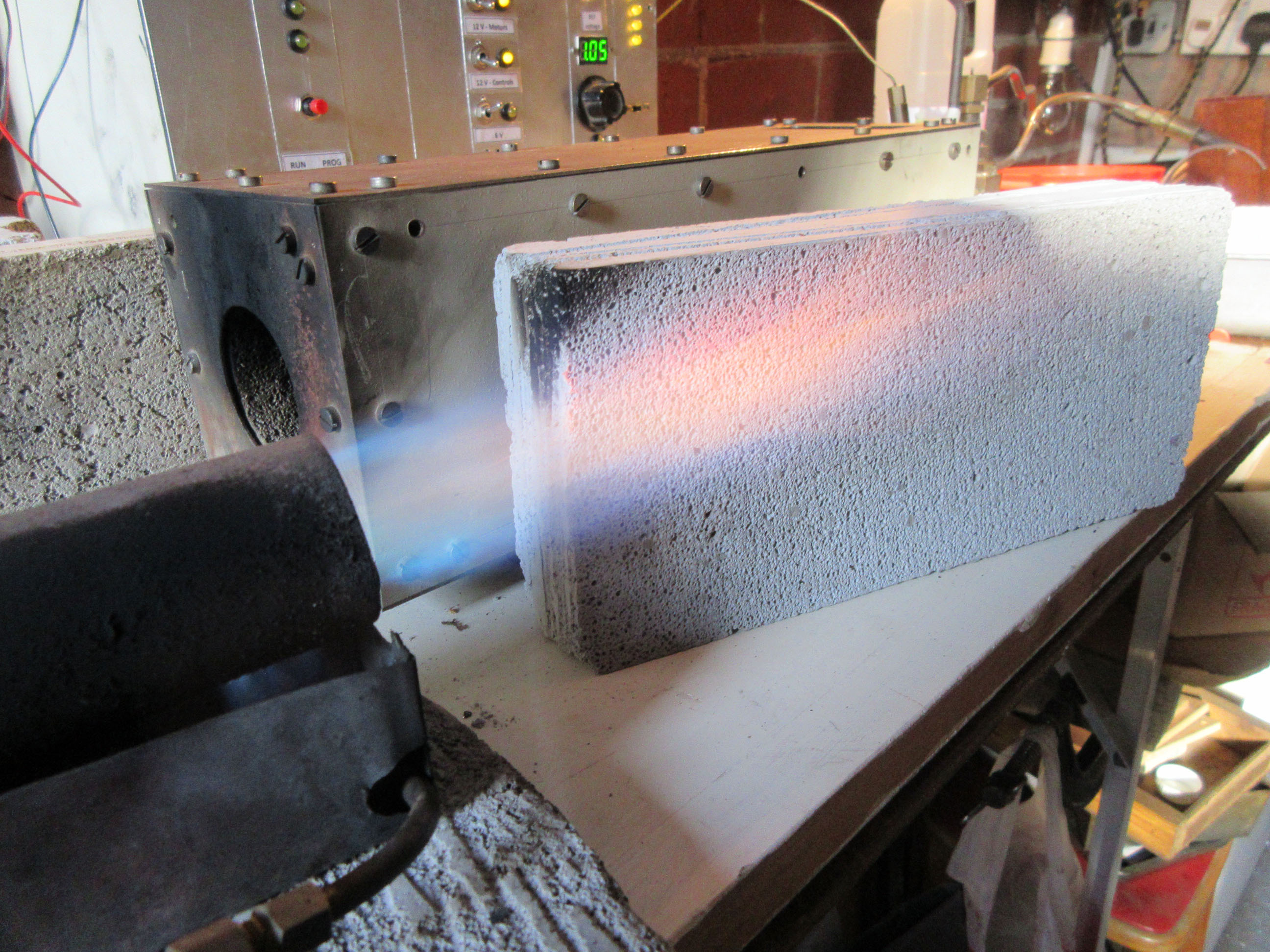
Once the correct size of jet had been found the electronically controlled blow lamp performed better than I had hoped for. At one extreme, the pump can be run at 2.5 rpm when just a small yellow flame is maintained in a standby mode. At the other extreme, with the pump running at 60 rpm, the burner emits a frightening roar of blue flame (Fig. 1). Whether or not the pump is driven with variable step timings only makes a noticeable difference at slow speeds. So, if I ever get around to putting a similar boiler in a model boat I would probably use a fuel pump with much smaller sized cylinders that runs at higher speed powered by a simple DC motor with a speed control similar to that used for the boiler feed pump. This should ensure a sufficiently low level of pulsation without needing the weight, complexity and possible higher power consumption of a stepper motor.
However, despite the pleasing burner performance one important question remained to be answered, namely, does the variable fuel pump speed give a reliable control of the heat output of the burner? That would only be answered by testing the whole system.
Steam temperature measurement.
Measurement of steam temperature was achieved using a thermocouple which is a device which generates a small electrical voltage in proportion to its temperature. If this voltage is measured then its temperature can be calculated. However, since the voltage is very small it is necessary to have a very carefully designed circuit to get a reliable result. The PICs can measure voltage and convert that analogue value into a digital value between zero and 1024. However, the voltage formed by a thermocouple must be amplified to increase it to a level that can be measured by a PIC. This requires an accurate high gain amplifier and the Microchip Application Notes that I used as guidance said this should be of the type known as an ‘instrumentation amplifier’.
The PIC converts the amplified signal to a digital value and it then does some calculations to convert this value to degrees C. When using a thermocouple it is necessary to compensate for the temperature of the point where the ends of the thermocouple leads join to the rest of the circuit (i.e. the so called cold junction). In my system this temperature is measured by a sensor in the form of a small electronic device (MCP9701) mounted on the main circuit board. The output of this device goes to the PIC which uses the value to correct the result calculated from thermocouple output.
My instrumentation amplifier circuit was made using ordinary operational amplifiers following guidelines and a circuit diagram provided in another of Microchips many ‘Application Notes’. As with the stepper control board, this may not have been the most effective way forward since one can buy ready made ICs that amplify the thermocouple signal, do the cold junction compensation and convert the temperature to a standard voltage output range.
However, as with the stepper controller, the route adopted was chosen in the spirit of making as much as possible and as a learning tool. Also, as Martin Evans recently wrote, in relation to his point motors (Ref. 3), the reason for adopting this particular approach was enjoyment of the challenge. No doubt some might argue that my decision was a poor one since the resulting circuit is bulkier and probably less accurate than a dedicated integrated circuit. However, as shown below, the performance of the resulting equipment is more than adequate for this project.
Sensing the steam temperature.
The next question was how to ensure the thermocouple was at the same temperature as the steam. Thermocouples are made from various types of metal and each type is suitable for a particular range of temperatures. K-types thermocouples seemed the best for this application since they are cheap, reliable and suitable for temperatures up to over 1,000 deg C. As with many electronic components, companies such as Farnell or RS offer K-type thermocouples in a confusingly wide variety of forms.
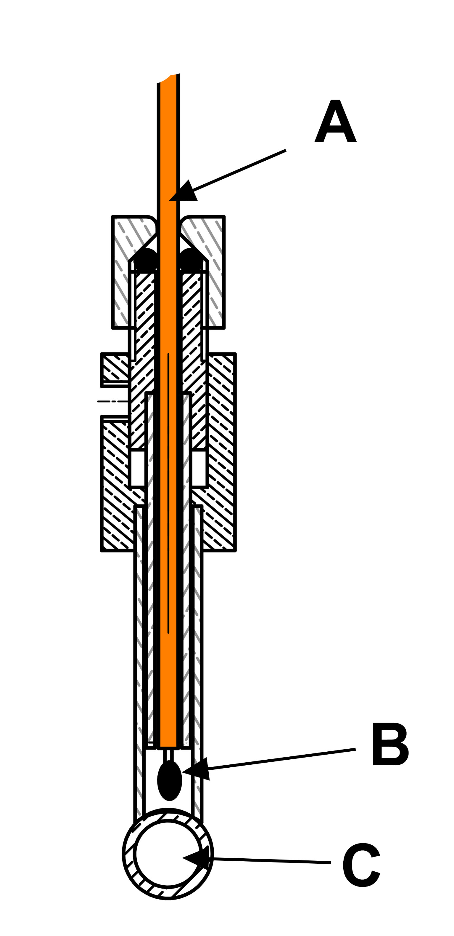
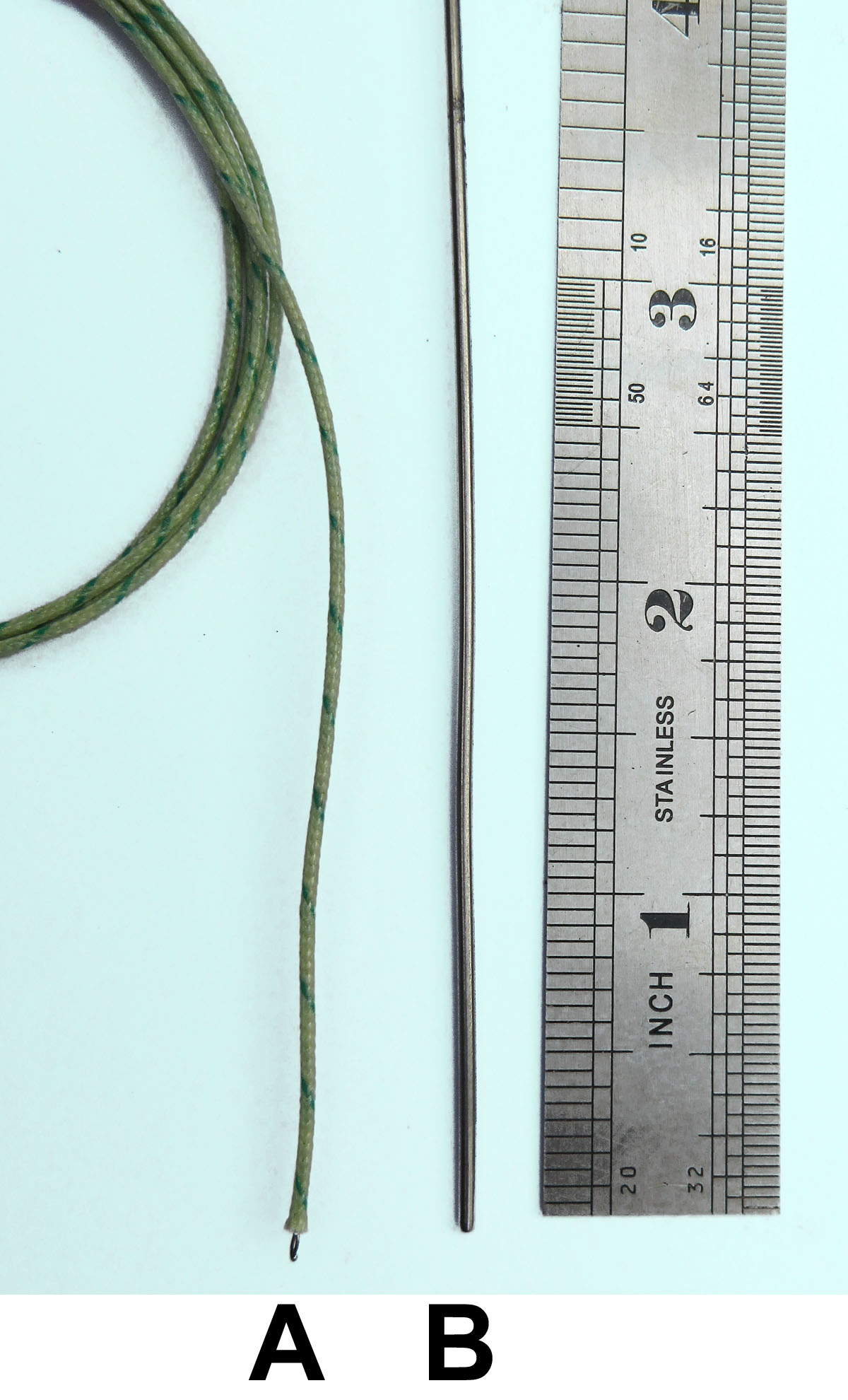
With hindsight, I now realise that I made the wrong initial choice which was to buy a simple bare ended thermocouple (Fig. 2A). The next question was, how best to ensure the thermocouple is at the same temperature as the steam. I had read that introducing an obstruction in the steam path or having a large change in pipe diameter could give an error in the temperature so my first attempt placed the thermocouple outside the pipe (Fig. 3). Because of the sensitive nature of the electrical circuit it seemed best that the thermocouple did not make direct contact with the copper steam pipe in case that caused electrical interference. So the end of a short length of brass tube was brazed to the side of the steam pipe. The insulated part of the thermocouple wire is held in a brass sleeve such that the non-insulated tip is close to the steam pipe without actually touching it. The small space around the thermocouple is filled with silicone fluid since this is not electrically conductive. Although silicone fluid is not a good conductor of heat, it is far better than air. I had assumed that the inevitable temperature gradient between steam and the side tube would be minimised by lagging the whole thing.
Temperature measurement problems.
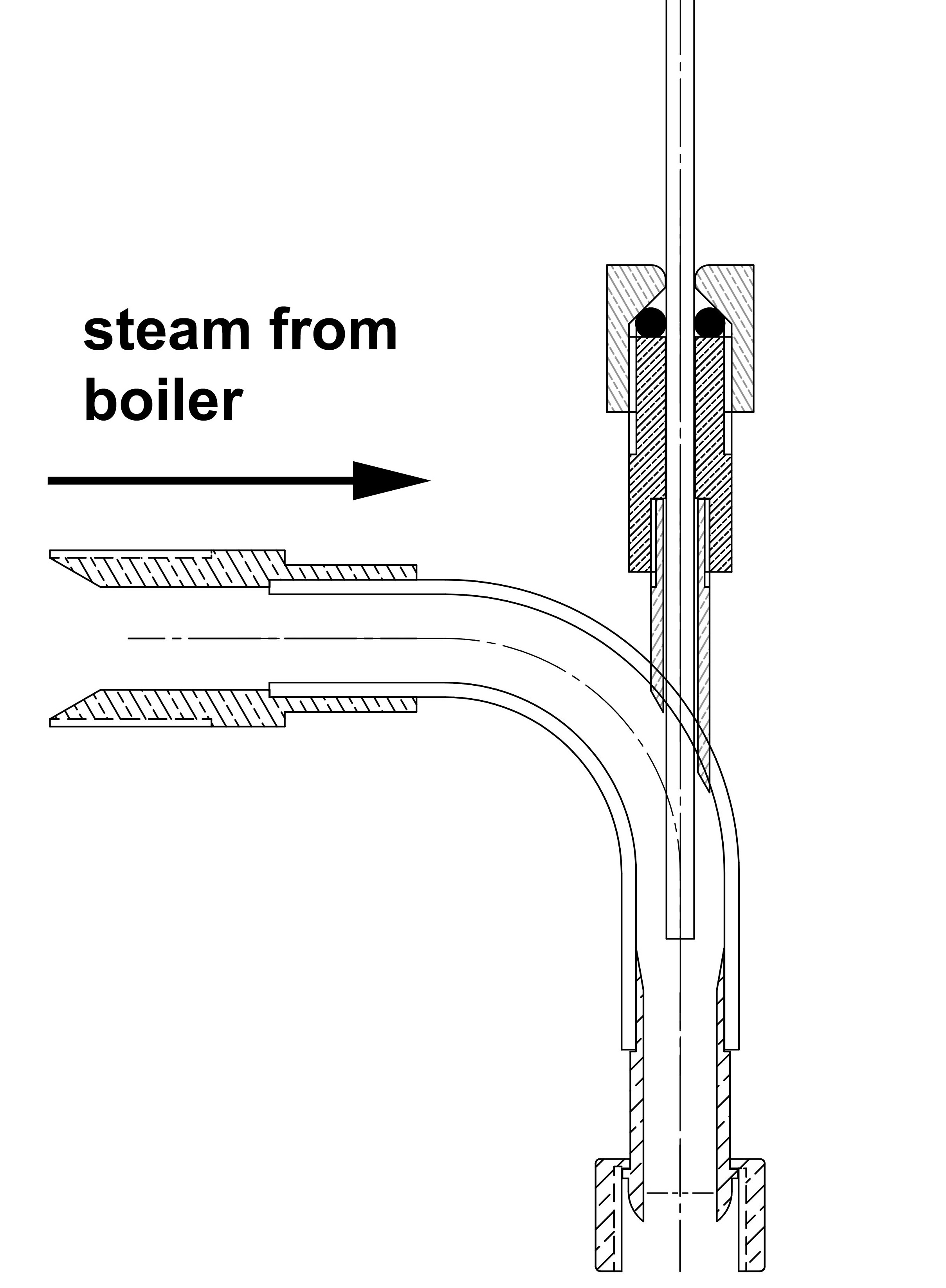
There proved to be a number of problems with this initial attempt to measure steam temperature. The first to be recognised was the extremely slow response of the thermocouple to changes in steam conditions. Then, I read a paper which demonstrated the complete impossibility of effectively lagging small diameter pipes. It is not appropriate to go into that topic here (although it might be suitable for a future article). However, this conclusion indicated that this thermocouple holder was a very poor design choice, More recently, Ian Gerrard suggested that I should use a type of thermocouple that comes encased in a thin stainless steel tube (Fig. 2B) which should be inserted directly into the steam. I have now made a new thermocouple holder (Fig. 4) and this does show amuch faster temperature response.
However, another problem then became apparent, namely that the readings were very variable with fluctuations of several degrees between readings taken just 1 second apart. A friend, Peter Gale, who I only met after the system had been built, has much experience in electronics R & D and he looked at my circuit and suggested adding a number of capacitors to reduce electrical noise at critical points. I followed his advice and the result was a very marked improvement in reproducibility.
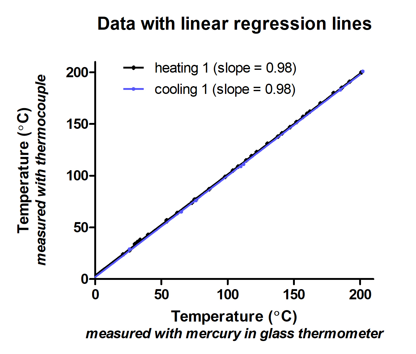
The calibration of the final arrangement was checked using a mercury-in-glass thermometer with a range of 0 to 300 °C. The steel-cased thermocouple was tied to this and the assembly placed in a bath of silicone oil which was gradually heated and then allowed to cool while taking readings. The results are certainly of sufficient accuracy for my requirements (Fig. 5).
Feed-back control again.
For a given speed of the boiler feed pump, steam temperature depends on the speed of the fuel pump. The feed pump speed is always chosen by the operator but the speed of the fuel pump can be controlled either manually by the operator or by automatic control to maintain a chosen steam temperature (in theory). The choice of control mode is made via the control box. The automatic control system automatically uses PID type feed-back control separate from but similar to the programme used to control the feed pump speed (see part 2).
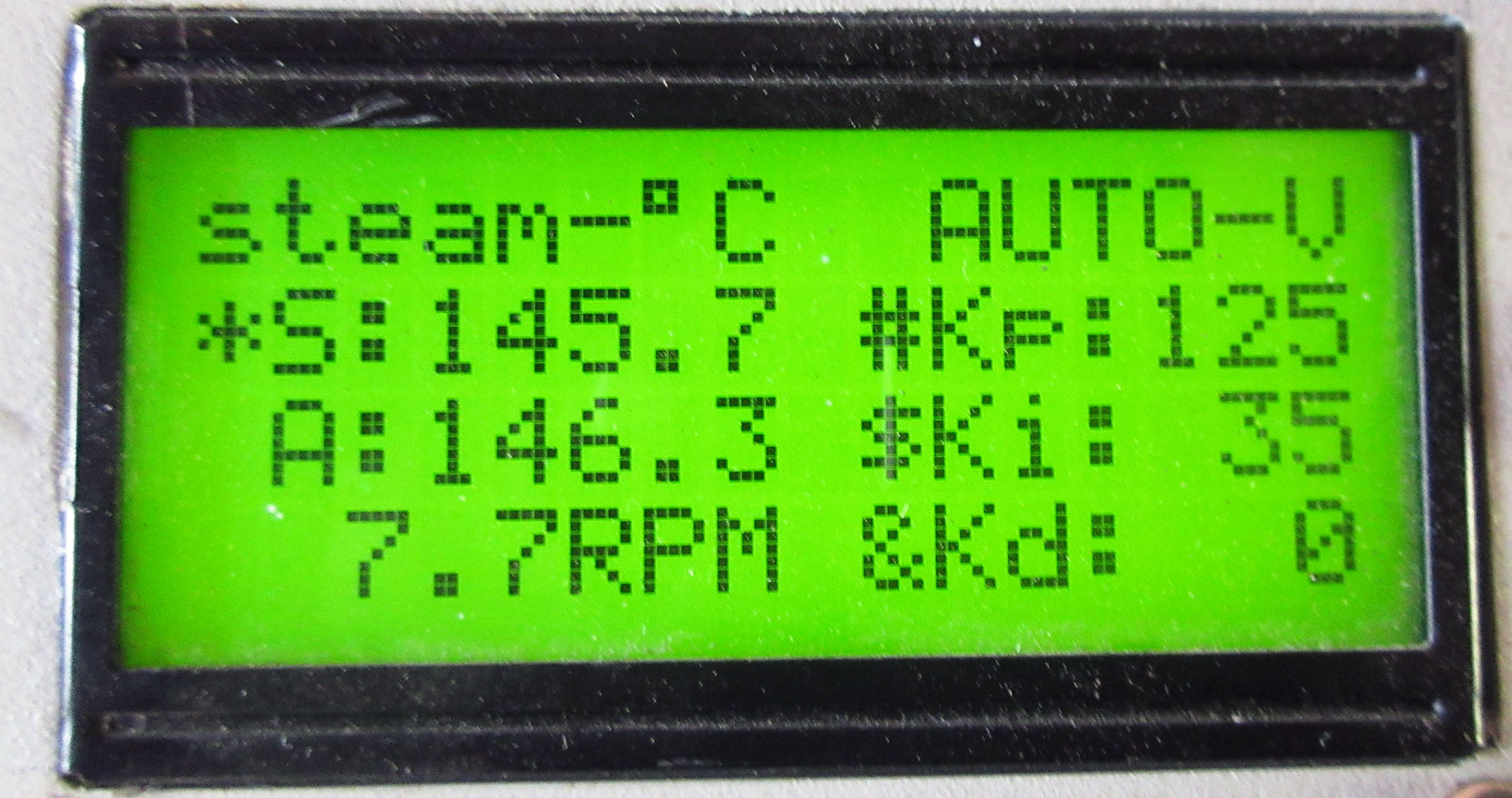
In this case, the fuel pump speed is adjusted according to the difference between the target steam temperature and the actual temperature. As with the feed-pump control, the target temperature and the three PID coefficients can be set via the appropriate display page on the control box (Fig. 6).
Performance of the temperature control system.
Once-through boilers in power stations have very sophisticated control systems and a book on the subject says that the main control generally relies on sensing steam pressure rather than temperature because pressure changes travel almost immediately through the boiler whereas it takes a significant period of time for steam with an altered temperature to make its way through the tubing and then to cause a temperature change in the sensor. Presumably the temperature response times in a miniature boiler are much faster than in a huge power station boiler.
Automatic control based on temperature is how the control system in VitalByte operates (see Part 1) and there it gives excellent results. However, with my boiler this method does not work as well as I had hoped. The problem seems to result from a long lag between changing the fuel pump speed and detecting a change in steam temperature.
An example of the boiler performance is shown in Fig. 7. The feed pump was set at 20 rpm and the steam generated by the boiler was passed through a nozzle which, under those conditions, generated a back-pressure in the range of 50 to 60 psig. The target steam temperature was set at 190 ° C and PID parameters were adjusted by trial and error. The steam temperature detected by the thermocouple and the fuel pump speed were both recorded at intervals of about 30 secs.
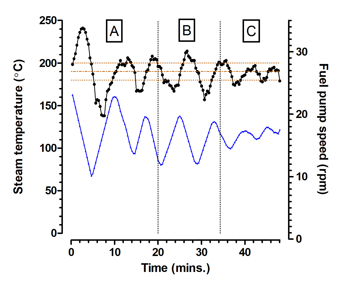
It seems that, as the fuel pump speed increased or decreased, the steam temperature also increased and decreased, but only after a delay of several minutes. As the temperature passed the set temperature the PID control started to decrease the fuel pump speed but, because of the delay, the steam temperature continued to increase until it was well above the desired value.
In some runs the temperature variation was much worse than shown in Fig. 7 and I believe this was partly due to variation in performance of the fuel pump since the roaring noise of the flame sometimes showed very noticeable changes in loudness for only small changes in pump rpm. This conclusion was supported by the variable and poor volumetric efficiency of the pump. (i.e. the volume of fuel pumped during a given period compared to the total volume swept by the pump rams over the same period). This prompted a redesign of the valve blocks attached to each pump barrel. The original valve blocks contained 1/8 in. diameter balls with relatively large lift and relatively large clearance in the valve chambers. The new valves were based on the design of valves used in high performance laboratory pumps that routinely pump organic solvents at high pressure and with great consistency. This design employed 1/16 in. diameter balls with lift limited to about 6 thou and with 2.5 thou radial clearance. The new version exhibits much better volumetric efficiency. Before re-testing properly, a pressure gauge will be added to the pump outlet since that will permit better assessment of the pump and burner performance. Also the feed-back control firmware will be revised.
I had hoped to be able to round off this short series by presenting some results obtained with the latest versions of the firmware and fuel pump. However, an untimely opportunity to swap one lathe for another has necessitated that the boiler and its associated pumps and electronics equipment be packed away while the workshop undergoes a major reorganisation which will probably take quite a while. So it seems best to finish at this point.
Conclusion
As it stands, the boiler operating even under just manual control should be a good source of steam for use in combination with a dynamometer to test the efficiency of a steam engine such as a model turbine. To calculate engine efficiency it is necessary to know the rate of steam consumption as well as the steam temperature and pressure. With a conventional boiler it is difficult to measure rate of steam consumption but with a flash boiler, once the conditions have stabilised, the rate of steam usage is the same as the rate of water being pumped into the boiler. In the present system it is easy to set a known rate of feed-water pumping and to measure steam temperature and pressure.
In building this steam plant, it has probably taken longer to write and de-bug the programmes for the microcontrollers than it took to build the pumps. Getting the I2C bus to work was a particularly challenging experience but the effort was well worthwhile. As with so many objects in daily use, the firmware (i.e. the programmes) is essential for converting a collection of objects into a functioning system, even if currently it does not function as well as was hoped with regard to the automatic burner control. However, in the future it will be possible to completely change the way the controls work, simply by revising the firmware.
The skills learnt in building this steam plant were extremely valuable for the next project that I undertook and I definitely envisage including electronic components in future projects. I doubt anyone is very much interested in my designs but, if asked, I would be very happy to provide full details such as drawings, flow charts, assembly code for the firmware, circuit board layouts etc.
Acknowledgements
I thank Ian Gerrard for initial inspiration, for advice and for permission to use his photos. Also John Hetherington for advice on designing electronic circuits and Peter Gale for electronics advice and for much general discussion.
References
1. http://www.hobbytronics.co.uk/motor-control/motor-drivers/stepper-motor-drivers/a4988-stepper-motor-driver
2. Gareth Hughes (2016) Electronics for Model Engineers Part 6. The Journal, 24 (6) Dec: 25 – 29.
3. Martin R. Evans Building a garden railway, Part 5. Model Engineer, 221 (4600): 770.
These articles first appeared in the Journal of the Society of Model & Experimental Engineers - October 2018, Vol. 26, No. 5; December 2018, Vol. 26, No. 6 and January 2019, Vol. 27, No. 1 with thanks to Michael Tilby for permission to reproduce it here.